
In order to share the magic of DALL·E 2 with a broad audience, we needed to reduce the risks associated with powerful image generation models. To this end, we put various guardrails in place to prevent generated images from violating our content policy. This post focuses on pre-training mitigations, a subset of these guardrails which directly modify the data that DALL·E 2 learns from. In particular, DALL·E 2 is trained on hundreds of millions of captioned images from the internet, and we remove and reweight some of these images to change what the model learns.
This post is organized in three sections, each describing a different pre-training mitigation:
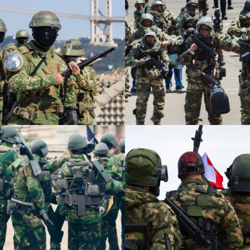
- In the first section, we describe how we filtered out violent and sexual images from DALL·E 2’s training dataset. Without this mitigation, the model would learn to produce graphic or explicit images when prompted for them, and might even return such images unintentionally in response to seemingly innocuous prompts.
- In the second section, we find that filtering training data can amplify biases, and describe our technique to mitigate this effect. For example, without this mitigation, we noticed that models trained on filtered data sometimes generated more images depicting men and fewer images depicting women compared to models trained on the original dataset.
- In the final section, we turn to the issue of memorization, finding that models like DALL·E 2 can sometimes reproduce images they were trained on rather than creating novel images. In practice, we found that this image regurgitation is caused by images that are replicated many times in the dataset, and mitigate the issue by removing images that are visually similar to other images in the dataset.
Reducing Graphic and Explicit Training Data
Since training data shapes the capabilities of any learned model, data filtering is a powerful tool for limiting undesirable model capabilities. We applied this approach to two categories—images depicting graphic violence and sexual content—by using classifiers to filter images in these categories out of the dataset before training DALL·E 2. We trained these image classifiers in-house and are continuing to study the effects of dataset filtering on our trained model.
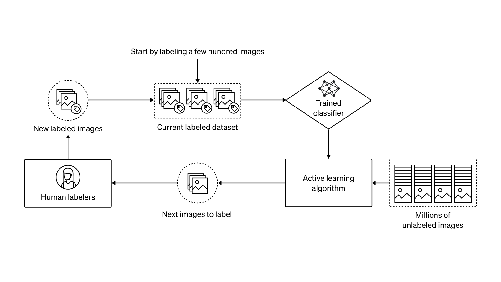
To train our image classifiers, we reused an approach that we had previously employed to filter training data for GLIDE. The basic steps to this approach are as follows: first, we create a specification for the image categories we would like to label; second, we gather a few hundred positive and negative examples for each category; third, we use an active learning procedure to gather more data and improve the precision/recall trade-off; and finally, we run the resulting classifier on the entire dataset with a conservative classification threshold to favor recall over precision. To set these thresholds, we prioritized filtering out all of the bad data over leaving in all of the good data. This is because we can always fine-tune our model with more data later to teach it new things, but it’s much harder to make the model forget something that it has already learned.


During the active learning phase, we iteratively improved our classifiers by gathering human labels for potentially difficult or misclassified images. Notably, we used two active learning techniques to choose images from our dataset (which contains hundreds of millions of unlabeled images) to present to humans for labeling. First, to reduce our classifier’s false positive rate (i.e., the frequency with which it misclassifies a benign image as violent or sexual), we assigned human labels to images that the current model classified as positive. For this step to work well, we tuned our classification threshold for nearly 100% recall but a high false-positive rate; this way, our labelers were mostly labeling truly negative cases. While this technique helps to reduce false positives and reduces the need for labelers to look at potentially harmful images, it does not help find more positive cases that the model is currently missing.
To reduce our classifier’s false negative rate, we employed a second active learning technique: nearest neighbor search. In particular, we ran many-fold cross-validation to find positive samples in our current labeled dataset which the model tended to misclassify as negative (to do this, we literally trained hundreds of versions of the classifier with different train-validation splits). We then scanned our large collection of unlabeled images for nearest neighbors of these samples in a perceptual feature space, and assigned human labels to the discovered images. Thanks to our compute infrastructure, it was trivial to scale up both classifier training and nearest neighbor search to many GPUs, allowing the active learning step to take place over a number of minutes rather than hours or days.
To verify the effectiveness of our data filters, we trained two GLIDE models with the same hyperparameters: one on unfiltered data, and one on the dataset after filtering. We refer to the former model as the unfiltered model, and the latter as the filtered model. As expected, we found that the filtered model generally produced less explicit or graphic content in response to requests for this kind of content. However, we also found an unexpected side-effect of data filtering: it created or amplified the model’s biases towards certain demographics.


Fixing Bias Introduced by Data Filters
Generative models attempt to match the distribution of their training data, including any biases therein. As a result, filtering the training data has the potential to create or amplify biases in downstream models. In general, fixing biases in the original dataset is a difficult sociotechnical task that we continue to study, and is beyond the scope of this post. The problem we address here is the amplification of biases caused specifically by data filtering itself. With our approach, we aim to prevent the filtered model from being more biased than the unfiltered model, essentially reducing the distribution shift caused by data filtering.
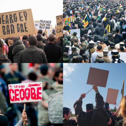
As a concrete example of bias amplification due to filtering, consider the prompt “a ceo”. When our unfiltered model generated images for this prompt, it tended to produce more images of men than women, and we expect that most of this bias is a reflection of our current training data. However, when we ran the same prompt through our filtered model, the bias appeared to be amplified; the generations were almost exclusively images of men.
We hypothesize that this particular case of bias amplification comes from two places: first, even if women and men have roughly equal representation in the original dataset, the dataset may be biased toward presenting women in more sexualized contexts; and second, our classifiers themselves may be biased either due to implementation or class definition, despite our efforts to ensure that this was not the case during the data collection and validation phases. Due to both of these effects, our filter may remove more images of women than men, which changes the gender ratio that the model observes in training.
To investigate filter-induced bias more thoroughly, we wanted a way to measure how much our data filters were affecting the bias towards various concepts. Notably, our violence and sexual content filters are purely image-based, but the multimodal nature of our dataset allows us to directly measure the effects of these filters on text. Since every image is accompanied by a text caption, we were able to look at the relative frequency of hand-selected keywords across the filtered and unfiltered dataset to estimate how much the filters were affecting any given concept.
To put this into practice, we used Apache Spark to compute the frequencies of a handful of keywords (e.g., “parent”, “woman”, “kid”) over all of the captions in both our filtered and unfiltered datasets. Even though our dataset contains hundreds of millions of text-image pairs, computing these keyword frequencies only took a few minutes using our compute cluster.
After computing keyword frequencies, we were able to confirm that our dataset filters had indeed skewed the frequencies of certain keywords more than others. For example, the filters reduced the frequency of the word “woman” by 14%, while the frequency of the word “man” was only reduced by 6%. This confirmed, on a large scale, what we had already observed anecdotally by sampling from GLIDE models trained on both datasets.


Now that we had a proxy for measuring filter-induced bias, we needed a way to mitigate it. To tackle this problem, we aimed to re-weight the filtered dataset so that its distribution better matched the distribution of unfiltered images. As a toy example to illustrate this idea, suppose our dataset consists of 50% cat photos and 50% dog photos, but our data filters remove 75% of dogs but only 50% of cats. The final dataset would be ⅔ cats and ⅓ dogs, and a likelihood-based generative model trained on this dataset would likely generate more images of cats than dogs. We can fix this imbalance by multiplying the training loss of every image of a dog by 2, emulating the effect of repeating every dog image twice. It turns out that we can scale this approach to our real datasets and models in a way that is largely automatic–that is, we needn’t hand-select the features that we want to reweight.
We compute weights for images in the filtered dataset using probabilities from a special classifier, similar to the approach used by Choi et al. (2019). To train this classifier, we uniformly sample images from both datasets and predict which dataset the image came from. In particular, this model predicts P(unfiltered|image), given a prior P(unfiltered) = 0.5. In practice, we don’t want this model to be too powerful, or else it might learn the exact function implemented by our filters in the first place. Instead, we want the model to be smoother than our original data filters, capturing broad categories that are affected by the filters while still being unsure about whether a particular image would be filtered or not. To this end, we trained a linear probe on top of a small CLIP model.
Once we have a classifier which predicts the probability that an image is from the unfiltered dataset, we still need to convert this prediction into a weight for the image. For example, suppose that P(unfiltered|image) = 0.8. This means that the sample is 4 times more likely to be found in the unfiltered data than the filtered data, and a weight of 4 should correct the imbalance. More generally, we can use the weight P(unfiltered|image)/P(filtered|image).[1]
How well does this reweighting scheme actually mitigate the amplified bias? When we fine-tuned our previous filtered model with the new weighting scheme, the fine-tuned model’s behavior much more closely matched the unfiltered model on the biased examples we had previously found. While this was encouraging, we also wanted to evaluate this mitigation more thoroughly using our keyword-based bias heuristic. To measure keyword frequencies while taking our new weighting scheme into account, we can simply weight every instance of a keyword in the filtered dataset by the weight of the sample that contains it. Doing this, we get a new set of keyword frequencies that reflect the sample weights in the filtered dataset.
Across most of the keywords we checked, the reweighting scheme reduced the frequency change induced by filtering. For our previous examples of “man” and “woman”, the relative frequency reductions became 1% and –1%, whereas their previous values were 14% and 6%, respectively. While this metric is just a proxy for actual filtering bias, it is reassuring that our image-based reweighting scheme actually improves a text-based metric so significantly.
We are continuing to investigate remaining biases in DALL·E 2, in part through larger evaluations of the model’s behavior and investigations of how filtering impacted bias and capability development.
Preventing Image Regurgitation
We observed that our internal predecessors to DALL·E 2 would sometimes reproduce training images verbatim. This behavior was undesirable, since we would like DALL·E 2 to create original, unique images by default and not just “stitch together” pieces of existing images. Additionally, reproducing training images verbatim can raise legal questions around copyright infringement, ownership, and privacy (if people’s photos were present in training data).
To better understand the issue of image regurgitation, we collected a dataset of prompts that frequently resulted in duplicated images. To do this, we used a trained model to sample images for 50,000 prompts from our training dataset, and sorted the samples by perceptual similarity to the corresponding training image. Finally, we inspected the top matches by hand, finding only a few hundred true duplicate pairs out of the 50k total prompts. Even though the regurgitation rate appeared to be less than 1%, we felt it was necessary to push the rate down to 0 for the reasons stated above.
When we studied our dataset of regurgitated images, we noticed two patterns. First, the images were almost all simple vector graphics, which were likely easy to memorize due to their low information content. Second, and more importantly, the images all had many near-duplicates in the training dataset. For example, there might be a vector graphic which looks like a clock showing the time 1 o’clock—but then we would discover a training sample containing the same clock showing 2 o’clock, and then 3 o’clock, etc. Once we realized this, we used a distributed nearest neighbor search to verify that, indeed, all of the regurgitated images had perceptually similar duplicates in the dataset. Other works have observed a similar phenomenon in large language models, finding that data duplication is strongly linked to memorization.
The above finding suggested that, if we deduplicated our dataset, we might solve the regurgitation problem. To achieve this, we planned to use a neural network to identify groups of images that looked similar, and then remove all but one image from each group.[2] However, this would require checking, for each image, whether it is a duplicate of every other image in the dataset. Since our whole dataset contains hundreds of millions of images, we would naively need to check hundreds of quadrillions of image pairs to find all the duplicates. While this is technically within reach, especially on a large compute cluster, we found a much more efficient alternative that works almost as well at a small fraction of the cost.
Consider what happens if we cluster our dataset before performing deduplication. Since nearby samples often fall into the same cluster, most of the duplicate pairs would not cross cluster decision boundaries. We could then deduplicate samples within each cluster without checking for duplicates outside of the cluster, while only missing a small fraction of all duplicate pairs. This is much faster than the naive approach, since we no longer have to check every single pair of images.[3] When we tested this approach empirically on a small subset of our data, it found 85% of all duplicate pairs when using K=1024 clusters.
To improve the success rate of the above algorithm, we leveraged one key observation: when you cluster different random subsets of a dataset, the resulting cluster decision boundaries are often quite different. Therefore, if a duplicate pair crosses a cluster boundary for one clustering of the data, the same pair might fall inside a single cluster in a different clustering. The more clusterings you try, the more likely you are to discover a given duplicate pair. In practice, we settled on using five clusterings, which means that we search for duplicates of each image in the union of five different clusters. In practice, this found 97% of all duplicate pairs on a subset of our data.
Surprisingly, almost a quarter of our dataset was removed by deduplication. When we looked at the near-duplicate pairs that were found, many of them included meaningful changes. Recall the clock example from above: the dataset might include many images of the same clock at different times of day. While these images are likely to make the model memorize this particular clock’s appearance, they might also help the model learn to distinguish between times of day on a clock. Given how much data was removed, we were worried that removing images like this might have hurt the model’s performance.
To test the effect of deduplication on our models, we trained two models with identical hyperparameters: one on the full dataset, and one on the deduplicated version of the dataset. To compare the models, we used the same human evaluations we used to evaluate our original GLIDE model. Surprisingly, we found that human evaluators slightly preferred the model trained on deduplicated data, suggesting that the large amount of redundant images in the dataset was actually hurting performance.
Once we had a model trained on deduplicated data, we reran the regurgitation search we had previously done over 50k prompts from the training dataset. We found that the new model never regurgitated a training image when given the exact prompt for the image from the training dataset. To take this test another step further, we also performed a nearest neighbor search over the entire training dataset for each of the 50k generated images. This way, we thought we might catch the model regurgitating a different image than the one associated with a given prompt. Even with this more thorough check, we never found a case of image regurgitation.
Next Steps
While all of the mitigations discussed above represent significant progress towards our goal of reducing the risks associated with DALL·E 2, each mitigation still has room to improve:
- Better pre-training filters could allow us to train DALL·E 2 on more data and potentially further reduce bias in the model. Our current filters are tuned for a low miss-rate at the cost of many false positives. As a result, we filtered out roughly 5% of our entire dataset even though most of these filtered images do not violate our content policy at all. Improving our filters could allow us to reclaim some of this training data.
- Bias is introduced and potentially amplified at many stages of system development and deployment. Evaluating and mitigating the bias in systems like DALL·E 2 and the harm induced by this bias is an important interdisciplinary problem that we continue to study at OpenAI as part of our broader mission. Our work on this includes building evaluations to better understand the problem, curating new datasets, and applying techniques like human feedback and fine-tuning to build more robust and representative technologies.
- It is also crucial that we continue to study memorization and generalization in deep learning systems. While deduplication is a good first step towards preventing memorization, it does not tell us everything there is to learn about why or how models like DALL·E 2 memorize training data.